This blog post has been adapted from a series of posts written for r/SimDemocracy. If you haven’t read the previous entries, please start with part 1.
In the last post, we went over how RRV extends SPAV to work with 0-n rated ballots. I mentioned that SPSV also extends SPAV to work with such ballots, but that it does so using a different method. In this post, I want to start off by explaining how this method works and why I find it superior to RRV’s approach. After this, we can move on to the full explanation of the motivation behind SPSV and to comparisons with other proportional methods.
Section A: The Kotze-Pereira transformation
The extension method that SPSV uses is called the Kotze-Pereira transformation, or KP transform for short. The basic idea behind the KP transform is that it’s possible to use approval ballots as building blocks for creating a score ballot. As an example, let’s use a 0-3 rated ballot that rates candidate A 0, candidate B 1, candidate C 2, and candidate D 3. We can construct this ballot out of 3 approval ballots by having the first ballot approve B, C, and D, the second approve C and D, and the third approve only D. That way, each candidate’s score equals the number of approvals they have.
This isn’t our only option though. We could also use 1 ballot that approves B and D, and 2 ballots that approve C and D. This is a problem because not only do we want to construct score ballots from approval ballots, we also want to decompose score ballots into approval ballots. Thus, we need a means of choosing a unique set of approval ballots for each score ballot.
It turns out that there’s a pretty intuitive criterion we can use. Specifically, we can restrict ourselves to only using approval ballots that “stack” on top of each other. By that, I mean there must be some way to order the ballots such that approvals are never added to subsequent ballots, only removed. Intuitively, this means that if each ballot was a row of toy blocks, then you could stack them on top of each other, like so:
| A | B | C | D |
|---|---|---|---|
| ✅ | |||
| ✅ | ✅ | ||
| ✅ | ✅ | ✅ |
In contrast, the second set of ballots cannot be stacked on top of each other:
| A | B | C | D |
|---|---|---|---|
| ✅ | ✅ | ||
| ✅ | ✅ | ||
| ✅ | ✅ |
If the approvals were toy blocks, the approval for B would need to floating in the air. If we try to solve this by moving the B and D ballot to the bottom, we find that the approvals for C would need to be floating. Thus, there is no valid way to stack these ballots.
It turns out that there is exactly one set of approval ballots that act as stackable building blocks for every possible score ballot. Constructing this set is simple: if a candidate receives n points from a score ballot, stack n approvals in that candidate’s column. Once you’ve done this for every candidate, the rows will form the desired approval ballots.
This is how the KP transform transforms a 0-n score ballot into n approval ballots. From here, it’s simple to describe how SPSV works: run the KP transform on every voter’s score ballot, then run SPAV on the resulting approval ballots. That’s it. That’s the entire voting method.
Section B: Comparison with RRV
It’s probably not clear whether the above process gives results that differ from those that RRV gives. However, since RRV and SPSV are considered different methods, you can probably guess that the answer is yes. It may not be immediately apparent what the differences are, but after exploring a simple example they should be much clearer.
First, let’s look at how electing a bunch of candidates that a voter slightly supports affects their ballot weight. We’ll consider an election with candidates A-G, where the voter rates A 5 and all other candidates 1. C will be elected first, then D, then E, and so on. We’ll look at how many points this voter’s ballot contributes toward both A and B as more candidates are elected, under both 0-5 RRV and 0-5 SPSV.
| Candidate | Method | N/A | C | D | E | F | G |
|---|---|---|---|---|---|---|---|
| A | RRV | 5 | 4.17 | 3.57 | 3.13 | 2.78 | 2.5 |
| A | SPSV | 5 | 4.5 | 4.33 | 4.25 | 4.2 | 4.17 |
| B | RRV | 1 | 0.83 | 0.71 | 0.63 | 0.56 | 0.5 |
| B | SPSV | 1 | 0.5 | 0.33 | 0.25 | 0.2 | 0.17 |
Let’s start with candidate A. Both methods start with the original score of 5. After C is elected, we can see that RRV has deweighted the ballot more harshly, going down to a 4.17 compared to SPSV’s 4.5. By the time G is elected, RRV has deweighted the ballot all the way to 2.5, while SPSV has only now reached 4.17. If we were to continue electing candidates with a rating of 1, RRV’s rating will approach 0 while SPSV’s rating will approach 4.
Moving on to candidate B, both voting methods start with a score of 1. The election of C prompts RRV to reduce the score to 0.83, while SPSV brings it all the way down to 0.5. Once G has been elected, RRV finally reaches 0.5, while SPSV is now all the way at 0.17. Continuing to elect candidates rated 1 would lead to both scores approaching 0, but SPSV’s score does so quicker than RRV’s.
This example shows that SPSV prioritizes preserving the strength of ratings for highly-preferred candidates, and deprioritizes preserving the strength of ratings for weakly-preferred candidates. This effect is strongest when the deweighting results from electing a weakly-preferred candidate. In contrast, RRV deweights all ratings equally, regardless of how preferred the elected candidate was. Personally, I think SPSV interprets my ballot in a more faithful way than RRV does, and I would guess that most people would feel similarly.
Section C: Visualizing representation accuracy
When it comes to choosing a good voting method, how faithfully it interpets ballots is not the only important factor to consider. We also want to take into account the accuracy of the voting methods in question.
In order to visualize this, I’m first going to have to set up the scenario in which the elections take place. In this scenario there are three factions: the cyan group, the magenta group, and the yellow group. There are three seats available, and each group is running three candidates. Every voter gives the same ratings to candidates if they are from the same group. Those ratings are as follows:
| Voter Group | Cyan Candidates | Magenta Candidates | Yellow Candidates |
|---|---|---|---|
| Cyan | 10/10 | 0/10 | 3/10 |
| Magenta | 7/10 | 10/10 | 0/10 |
| Yellow | 0/10 | 5/10 | 10/10 |
At this point, the only detail we haven’t covered is the distribution of the three groups of voters. I’ve saved this for last because we actually won’t be looking at a single distribution of the three groups, but rather all of them.

This is an example of a ternary plot. This particular ternary plot shows the proportion of the electorate that each group makes up. In the top-left corner, the electorate consists of only cyan voters. In the top-right corner, the electorate consists of only magenta voters. And if you couldn’t guess, in the bottom corner the electorate consists of only yellow voters. As you move closer to the center, the mix of voters becomes more even, until you reach the center where each faction makes up exactly 1/3 of the electorate.
Now that you’ve seen the voter distribution, we’re going to look at what the winners look like for each of these possible electorates. We’ll start with a method we covered a while back, D’Hondt. Since D’Hondt uses single-mark ballots, each group will simply vote for a candidate from their faction. The distribution of winners looks like this:

Here, the colors represent how many candidates were elected from each faction. In the top-left, all elected candidates were from the cyan faction, so the area is colored cyan. Below that, we see a greenish-aqua color. This represents the election of two cyan candidates and one yellow candidate. If we then move to the right, we see a gray area that represents the election of one candidate from each group.
As you can see, D’Hondt behaves pretty nicely when voters can easily be divided into factions. However, because it uses single-mark ballots, it cannot take into account anything other than voters’ first preferences. Thus, even in this favorable scenario it still can’t behave optimally.
Next, we’ll take a look at how RRV behaves.

There are a couple things to notice here. First of all, this plot doesn’t look nearly as nice as the one for D’Hondt. This is pretty much an inevitable result of using information beyond first preferences. However, RRV actually doesn’t do that bad, all things considered. If you’re curious, you can check out how other proportional rated methods perform for yourself; you’ll see that many of them have larger concave areas and appear far more irregular than RRV does.
Moving on, the other thing to notice is that the plot is no longer symmetrical. Looking at the corners, the cyan area is larger than the other two, and the yellow area is the smallest. This reflects how the cyan candidates each receive 7 points from every magenta voter, and thus have a lot of second-choice support. Yellow, on the other hand, has very little second-choice support, and this is reflected in its smaller area.
The last method we will look at is, of course, SPSV. Here is its plot:

Overall, it looks pretty similar to RRV’s plot, which makes sense given that they are both extensions of SPAV. The main difference is that the center region is larger while the corner regions are all smaller. In fact, SPSV’s regions vary in size less than RRV’s do. The variance between the different corners hasn’t changed much, since SPSV still takes second choices into account. However, RRV had an oddly small center region, indicating that it is biased toward only representing two factions.
This is easier to observe if we increase the number of seats available. Below are the plots for RRV and SPSV when filling 10 seats instead of 3.
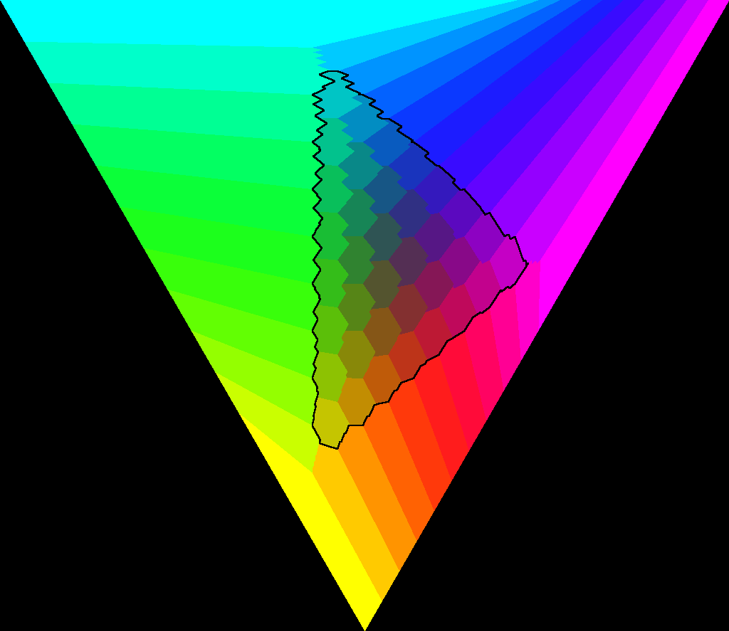
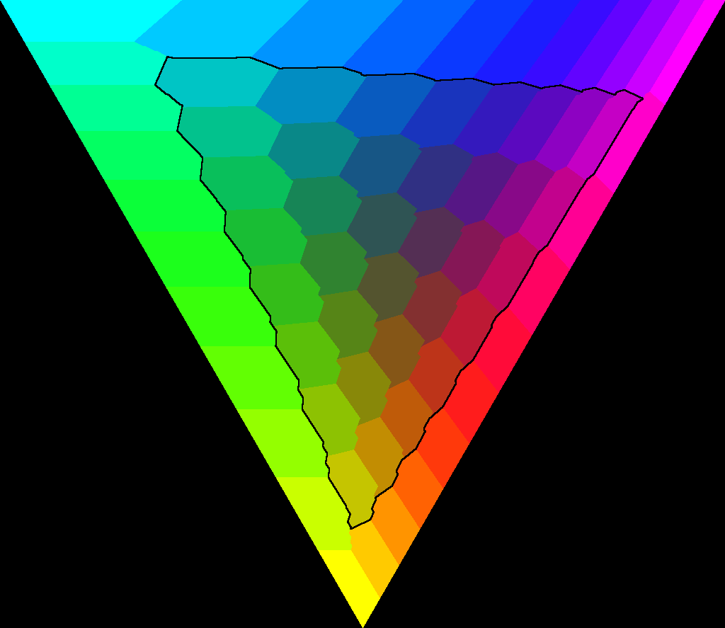
As you might’ve guessed, the top plot is for RRV while the one below is for SPSV. The region outlined in black on each plot is the area in which all 3 factions have at least one candidate elected. In RRV, this area is really small, around 1/4 the size of the whole ternary plot. In SPSV, this area takes up all but the outer edge of the plot. A faction will only be completely excluded by SPSV if it makes up a really small proportion of the population, in which case there simply aren’t enough seats to fairly include them.
I hope that everyone reading this feels that they have a better understanding of SPSV, or at least enjoyed themselves along the way. I know that this stuff can seem very complicated, and I’m not always able to explain things well. I encourage you to comment below with any questions you may have, and I’ll do my best to make things clearer. Thank you for reading! ❤️